
In the past few years, I’ve moved more than once. Time and again, I have had to measure rooms or furniture and then check whether I can arrange everything just as I had planned. When we use a tape measure, folding rule or ruler, we don’t question whether the object we are measuring is measurable. As long as something is not infinitely extended, we should be able to assign it a length, area or volume. That is exactly what mathematicians assumed—until the late 19th century, when everything changed.
For a long time, if you wanted to measure geometric objects, you proceeded as I did when moving house: take out the tape measure and off you go. Admittedly, if you wanted to determine the area underneath a complicated curve, the task became more difficult. With the development of calculus in the 17th century, mathematicians Isaac Newton and Gottfried Wilhelm Leibniz provided new measuring instruments in the form of integrals and derivatives that could be used to precisely determine the size of geometric figures. But for more than 200 years, nobody really asked themselves how objects should be measured.
At the end of the 19th century, when experts attempted to cast mathematics on a stable foundation, set theory became the cornerstone. This theory puts forward that everything—including geometric shapes and complex differential equations—can be traced back to elementary sets. But if geometric shapes are nothing other than sets, then we must find out how to measure abstract sets.
On supporting science journalism
If you’re enjoying this article, consider supporting our award-winning journalism by subscribing. By purchasing a subscription you are helping to ensure the future of impactful stories about the discoveries and ideas shaping our world today.
Let’s take the interval on the number line between 0 and 1, which is written as [0, 1]. It contains an infinite number of real numbers, but, for our purposes, let’s say its length corresponds to one centimeter. Mathematicians like to calculate without units and therefore define that the interval [0, 1] has the length 1. Similarly, the interval [0, 2] has a length of 2, and so on.
Of course, experts did not simply decide this but instead derived it according to certain rules. To establish these rules, they tried to summarize all the intuitive properties that a measure such as length, area or volume should have. Namely, the measure of the empty set should be zero; the measure of an object does not change when you move the object; and the measure of nonoverlapping objects is equal to the sum of the measures of the individual objects. From these three simple conclusions, various dimensions can be defined, including the above-mentioned length dimension, which corresponds to our intuition.

To calculate the measure of nonoverlapping sets, you can add the measures of the individual sets.
The procedure may seem rather cumbersome: after all, you knew the result intuitively. This approach makes it possible to measure quantities more broadly, however, even those for which there is no geometric conception.
A Measure for Abstract Quantities
When mathematicians first became interested in measures, they initially studied functions (that is, the expression or rule that defines the relationship between two variables, x and y). You may remember from secondary school that you can determine the area below a function by integrating it. For example, you might use the Riemann integral, in which you form upper and lower sums to determine the area under a curve. See, for example, the blue bars in the image below, which represent how the x axis can be divided into small intervals that can be added together to calculate the total area.
But what happens if the function is extremely complicated? If you look at the fragmented Dirichlet function, for example, you don’t get very far with the usual integral concept. The Dirichlet function χ(x) has the value 1 if x is a rational number. Otherwise the function’s value is always zero. Graph this function and you will see that χ(x) consists of an infinite number of points along the line y = 1 and y = 0. Because the graph of the function only consists of individual, disjointed points, it is impossible to use the Riemann integral.
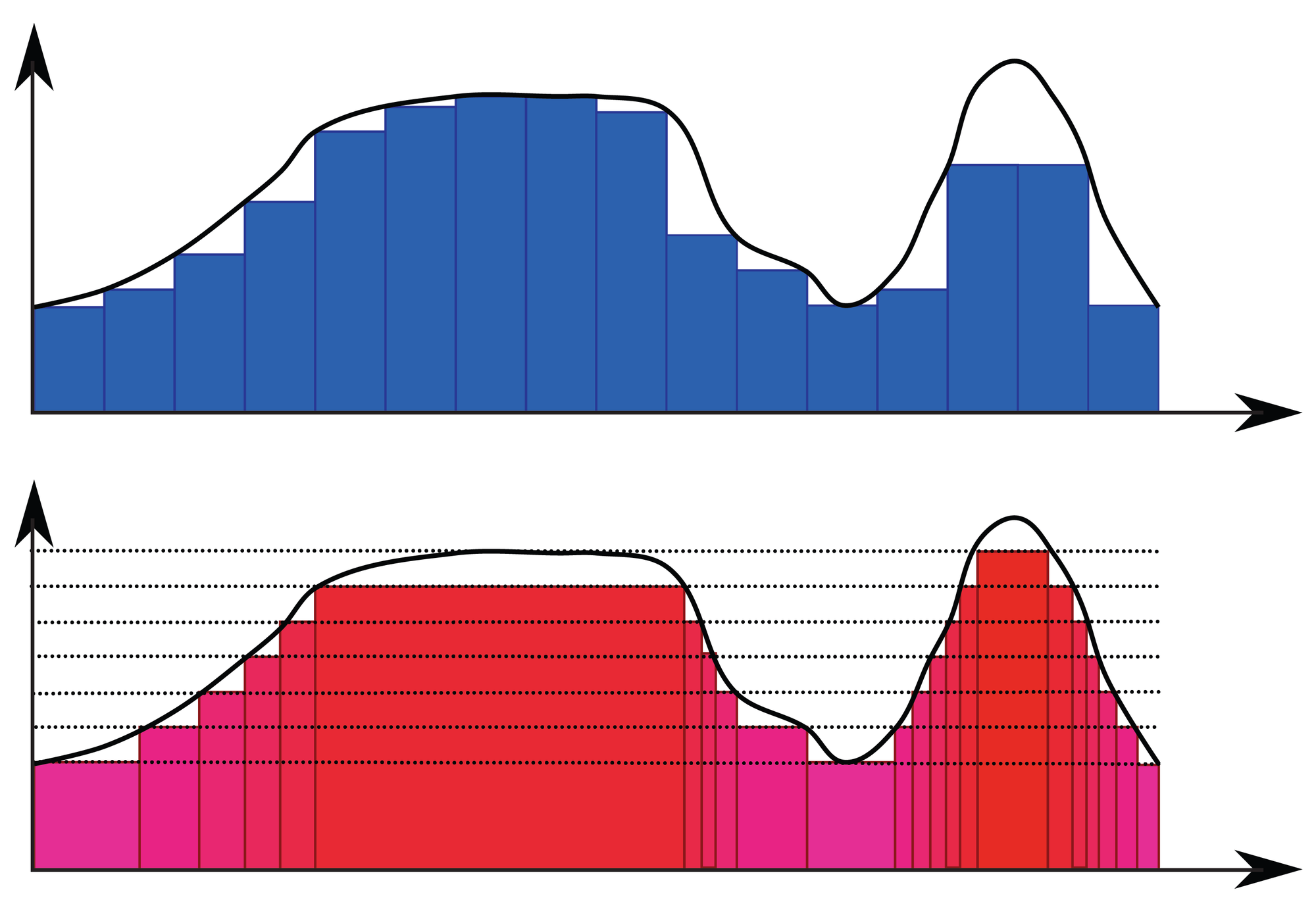
The Riemann and Lebesgue integrals each define integrals by breaking them down, The Riemann integral breaks them down vertically (blue), and Lebesgue breaks them down horizontally (red).
Svebert/Wikimedia Commons (CC0 1.0)
Instead you need to turn to the Lebesgue integral, introduced by mathematician Henri Lebesgue in 1902. In this case, the y axis is divided into small intervals—as in the red bars in the image above. To calculate an area, you must determine the width of the corresponding intervals on the x axis.
For all ordinary functions that are not as fragmented as the Dirichlet function, the Lebesgue integral and the Riemann integral provide exactly the same result. The advantage of the Lebesgue integral is that it can also assign an area to more complicated cases.
So to return to the Dirichlet function, in the interval [0, 1], let’s use the Lebesgue interval and divide the y axis into small sections. The points of the function only lie at y = 0 for an irrational x value or y = 1 for a rational x value, so the result is 0 times the length of all irrational numbers in the range [0, 1] plus 1 times the length of all rational numbers in [0, 1]. At this point, we need measure theory to assign a length to the abstract sets: the irrational numbers between [0, 1] and the rational numbers between [0, 1]. Because there are only countably many rational numbers (see the image and caption below for a proof of that statement), their measure is zero. The measure of the remaining irrational numbers between [0, 1] must therefore be 1 (because all real numbers in [0, 1] together have the measure 1). The area below the Dirichlet function between zero and one is therefore 1 x 0 + 0 x 1 = 0.

Consider the set M = {m1, m2, m3, …, mi, …}. Because M contains countably many elements, they can be numbered with an integer index i. To determine the dimension μ(M), one can make an estimate. To do this, form a small interval Ii around each mi with a decreasing, arbitrarily small width ε/(2i): Ii = [mi − ε⁄(2i+1), mi + ε⁄(2i+1)] and form one from it new set C = {I1, I2, I3,…, Ii, …}. So C is similar to the original set except that it does not contain individual points m but rather small intervals. Overall, the measure of C would have to be at least as large as the measure of M: μ(M) ≤ μ(C). Now the measure of C can be calculated by assuming that ε is chosen so small that the intervals Ii never overlap. The measure then corresponds to the added lengths of the intervals: μ(C) = ∑i∞ε/(2i) = ε. This means that the measure of M must be less than or equal to ε: μ(M) ≤ ε. Because ε can be chosen to be arbitrarily small, the measure of M must result in zero. This proves that for every countable set, μ(M) = 0 holds.
Manon Bischoff/Spektrum der Wissenschaft
The Measurement Problem Appears
The Lebesgue integral gave rise to the so-called measurement problem in 1902. Experts wondered whether it was possible to assign a measure to every quantity. And just three years later mathematician Giuseppe Vitali came up with a sobering answer: no, there are sets that are so jagged that they cannot be measured.
Vitali came to this realization when he constructed a concrete set for which any kind of measure fails: the Vitali set, named after him. He started simply and considered the set of all numbers between 0 and 1. He then divided this set into different areas: two numbers a and b end up in the same range if a – b results in a rational number. For example, all natural numbers and all rational numbers are in the same region. In another region, there are 0,2 + √0,2 and 0,3 + √0,2, and so on. Vitali thus divided the interval [0, 1] into (uncountably) infinitely many small parts.

To construct the Vitali set, decompose the interval [0, 1] into individual regions. Two numbers (pink and purple circles) are in the same range if their difference results in a rational number.
Manon Bischoff/Spektrum der Wissenschaft
In the next step, he selected exactly one representative r from each of these ranges and inserted all these representatives into a new set V. The set V thus contains an uncountably large number of elements because there are an uncountably infinite number of subdivisions of the interval [0, 1]. Then Vitali turned to a trick: he investigated what happens if the set V is shifted by a rational number p, which assumes a value between [–1, 1]: Vp = V + p. As a result, the rational number p is added to every element r in V. In this way, Vitali generated a countably infinite number of sets Vp that contain numbers between [–1, 2]. The reason for this is that V contains numbers between [0, 1] and p adds values from the interval [–1, 1].
This is all pretty technical, but don’t worry; we’re almost there! The Vitali set V* contains all Vp and, as we will see, goes beyond the concept of measure theory. We know that the measure of V* is at least as large as the measure of the interval [0, 1] (because V* is at least as large as V, which has a range from 0 to 1). On the other hand, the Vitali set is smaller than or equal to the interval [–1, 2]. This means μ ([0, 1]) = 1 ≤ μ(V*) ≤ μ([–1, 2]) = 3. Accordingly, the Vitali set must measure between 1 and 3.
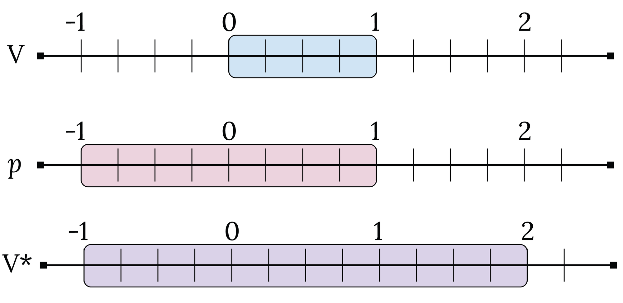
The set V ranges from 0 to 1, while the values p range from –1 to 1. Therefore, the Vitali set V* extends from –1 to 2.
Manon Bischoff/Spektrum der Wissenschaft
Now you can also calculate the measure of the Vitali set directly: μ(V*) = ∑pμ(Vp) because there are only countably many p. The set Vp contains an uncountable number of elements between [p, 1 + p], however, so that μ(Vp) is a finite number greater than zero. And in fact, all Vp are the same size—different values of p only represent a shift, which is irrelevant for the size of a set. This means μ(Vp) = μ(V). Accordingly, the measure of the Vitali set is μ(V*) = ∑pμ(V), i.e. a constant μ(V) that is summed infinitely often. The result of such a calculation is always infinite—regardless of how small the constant μ(V) is. This means: μ(V*) = ∞, which contradicts the above inequality 1 ≤ μ(V*) ≤ 3.
There Will Always Be Nonmeasurable Quantities
The surprising result does not mean we have done the math wrong. Rather, the Vitali set is so complex that no measure can be assigned to it. Vitali thus proved that not all quantities are measurable; there are also “nonmeasurable” quantities.
That result in itself is astonishing. After all, the Vitali set is limited and only contains real values. If you transfer this result to two-dimensional sets, you get even stranger results: for example, you can double the surface area of a sphere by decomposing it into nonmeasurable sets.
Fortunately, nonmeasurable quantities are extremely rare. In physics, for example, they do not occur—after all, decompositions of objects are limited by the size of atoms. You have to construct nonmeasurable quantities in order to come across them. And yet they are omnipresent: even in simple numerical intervals, nonmeasurable sections lurk. As it turns out, it is not so easy to get rid of such quantities. One would have to change the axioms—and thus the foundation—of mathematics to prevent the occurrence of nonmeasurable quantities.
This article originally appeared in Spektrum der Wissenschaft and was reproduced with permission.